How AI works, plain English, no math
There might be a few diagrams, but I promise they aren't scary.
I’m pretty convinced modern AI will be a world-transforming technology on the same scale as, say, smartphones. As such I think it’s important that non-technical people understand how and why it works … but this is much harder for AI than it was for smartphones. People intuitively understand “small computers connected by radio waves.” But attempts to explain modern machine learning are frequently built around concepts and math so intimidating they repel even experienced software engineers, much less the general public.
My goal here is to explain to a broader audience — readers who don’t know calculus — how neural networks (the technology behind AI) work, in particular OpenAI’s DALL-E image generator, in reasonably thorough and rigorous detail, with a few simple illustrative diagrams … but no math, and no unexplained mathematical terms, whatsoever. Wish me luck. (Of course one reason I’m writing this is to force myself to understand the subject much better myself.)
[Terminology note: by DALL-E I mean the image generator at labs.openai.com. At one point this generator was called “DALL-E 2”, to distinguish it from its alpha release. To avoid further nominative confusion, let’s pretend that initial version never existed.]
i. Signal to Denoise
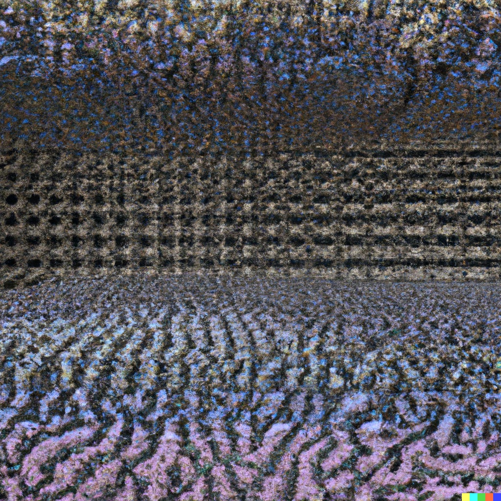
The engine at DALL-E’s heart is fascinating; it literally uses meticulous computation to conjure order out of chaos. Training DALL-E initially consists of taking a huge number of existing images and then, bit by bit, adding “noise” to them, i.e. scrambling them, so that they’re first mostly recognizable, then very staticky, and finally indistinguishable from random noise. Turning order into chaos.
But the key is to make this process reversible, meaning that the system learns how to invert the order of operations, and turn chaos into order. Specifically, it learns how to begin with random static and slowly “denoise” it, step by step, into a high-quality image. Then, at every step, it gently nudges this “denoising” process in directions suggested by the text the user entered, so that the initial chaos is gradually ordered into a high-quality illustration of the user’s prompt.

I hope you’ll agree that the above is both a captivating idea and a powerful metaphor. (Practitioners may think of it more as a mathematical trick — turning a function not susceptible to efficient computation into one which is — but let’s not miss the metaphorical forest for the mathematical trees.) It’s an accurate depiction of what DALL-E does … but it’s also very vague and handwavey. What exactly do we mean by “noise”? How do you train a system to “denoise”? In fact, what does “training” even mean? Once it’s trained, how does this “nudging” work? What other details are we eliding from this oversimplification? Again, this is very likely the world’s next most important technology. It behooves us to go at least a little deeper. To do so, let’s first back out a bit, and begin with the basics.
ii. What even is a neural network?
Before looking inside neural networks, let’s just consider their inputs. Those are simply a bunch of numbers. Those numbers can represent text, an image, sound — anything, really — but to the network, they’re just a group of numbers it will ultimately transform into a different group of numbers. The interesting part is how. Unlike traditional computers which run software, neural networks use neurons.
Those neurons are loosely based on those in our brains, but please don’t think that makes neural networks a lot like brains; they aren’t. (This is one reason practitioners sometimes use the word “perceptron” instead. We’ll stick with “neuron.”) To visualize a neuron, just imagine a little black box with a bunch of lines going into it, and one line coming out. The ones going in are its inputs, which are just numbers, and the one coming out is an output, also just a number. A very simple neuron might merely add up all its inputs and output that sum.
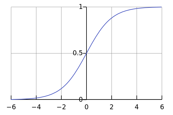
In practice, though, if you imagine every input coming in through its own individual slot, each slot is given an adjustable weight, indicating how much its particular input should be multiplied by. Then the neuron’s output value is dictated by some sort of output function, usually a curve like the one below. When it “fires,” it adds up all its weighted inputs, and outputs the height of the curve associated with that total. So, for example, if a neuron with the output function below had its weighted inputs add up to precisely 0, it would output 0.5. If they added up to 6, it would output more like 0.999. That’s it, that’s all, pretty simple.
It’s pretty amazing that today’s dizzyingly powerful AI systems are created from such a basic building block. The secret is having a very large number of such neurons, carefully connected and exhaustively trained. In practice, neural networks — i.e. networks of neurons — are almost always arrayed in layers, with data flowing from each layer to the next:

There are usually many more layers, each often numbering in the thousands of neurons — but the same principle applies. A reasonably good analogy is to envision water falling down a staircase; the data is the water, and the layers are the steps.
What’s remarkable about neural networks is that the steps can be shaped, or trained, so that the “water” pools, collects, and intermixes in such an extraordinarily precise and powerful way that in the end something amazing happens — like a recognizable human face appearing at the final step. At heart, it’s just an agglomeration of quite basic math, as described above! But the results sometimes feel like magic.
iii. Feed forward, propagate back
Of course in reality data has no “gravity,” and can metaphorically run uphill; but many of today’s useful neural networks are feedforward, meaning their data flows only in one direction. Even those where it loops back around, known as recurrent networks, can often still be usefully modeled in terms of unidirectional data. It’s also common for some data to jump two or more layers at once, just as channels cut into the side of our waterfall could allow some water to skip steps; these are known as skip connections.
It turns out that if a neural network is sufficiently well designed, and its layers are big enough, dense enough, and sufficiently well constructed — millions of neurons and billions of weights, set with incredible precision — then its resulting complexity can contain extraordinary recognitive and transformative powers, such as understanding text prompts and generating corresponding images. The obvious question is: how can we set those weights to achieve that incredible power and precision?

The answer is: a) very gradually b) at enormous computational expense. Neural nets are not programmed with written software code like “normal” computers. Instead they are trained — which is to say, their weights are slowly tweaked and refined, many many times, each iteration nudging them a little further towards their optimal levels. The secret to training them is finding a way to mathematically express the difference between what the neural network currently does, and what you want it to do. This expression is known as the “loss function” or “cost function.” (Don’t worry, we won’t show any. This is a safe, math-free space.) Given a good loss function, you can take what the network outputs now; compare it with what you want; and then determine which direction to “push” each individual weight in the network so that the overall output gets closer to the desired result.
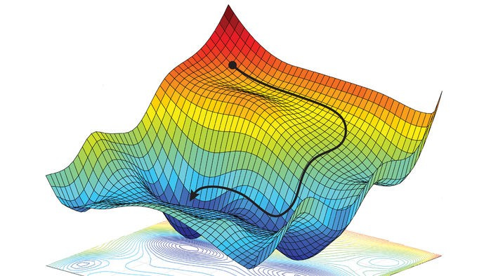
For instance, to train your neural network you might give it a slightly noisy picture of a cat. What you want it to output, once fully trained, is a cleaned-up, less noisy picture of that same cat; but what you’ll actually get, early in the training, is just a blob of random colors. The magic of a well-behaved loss function is that can show you which direction to shift every individual weight in the network to improve its overall results. This direction is known as the gradient, and this approach to training is called gradient descent. (“Descent” because the “loss function” basically describes how bad/wrong the output is, so you want its values to go down over time.)

In practice, gradient descent is generally performed with a technique known as backpropagation, which lets you train networks very efficiently. This consists of first measuring the final outputs, and using those to work out how to tweak the last layer’s weights; then looking at the outputs of the second last layer, and tweaking its weights accordingly; then moving on to the third last layer; etcetera. With backpropagation, each training iteration consists of running data through the network, measuring its outputs, and then going backwards through it, adjusting one layer at a time, so that its next training run works a little better.
Note that we can determine the direction of the weight changes we want, and a rough sense of how much each change will affect the output … but not exactly how much to change each weight. That’s why you do many training runs, tweaking each weight a little bit at a time, finding your way slowly to the minimum of the loss function. Gradient descent is a bit like skiing in dense fog; at any given moment, you know how steep the slope is where you are, but not what the territory ahead looks like, or if there are hills between you and the promised land of the lodge. If we change too much, we can go past an optimum level and have to double back, possibly repeatedly; but if we change too little, we can go down blind alleys and/or training can take much longer than necessary. Setting the appropriate rate of change, known as the learning rate, is something of a judgement call.

Pushing our waterfall-over-stairs analogy to its limits — but it still holds — you can think of training a neural network as pouring a bucket of water down the stairs; checking to see whether it pools at the bottom in the way you want; and then following the water back up the stairs, examining the patterns en route, and carving the edges of the steps accordingly, one at a time, using a set of tools whose precision is determined by the learning rate … all so that the next bucket will perform better. If you have a good loss function, and you chose the right number and kind of steps and side channels, and a good learning rate, then eventually, inexorably, the magic will happen. But as any machine learning engineer will tell you ruefully, there are many, many ways training can go wrong.
iv. To be continued
You (hopefully) now have a reasonably good understanding of how modern AI works in general. But of course it gets more complicated. There are a whole slew of different types of neural network: convolutional, generative adversarial, long short-term memory, variable autoencoder, transformer, and many more, each with its own application(s). Most fit the description above reasonably well … but details matter. In Part 2 of this post, we will zoom in on how DALL-E, specifically, works.


